This post is a quick introduction to genetic algorithms. I will describe all the steps required for such an algorithm to work, explain concepts, and show an example of implementation in Python.
What is a genetic algorithm?
The genetic algorithm (GA) is a heuristic method that can find the optimal solution for the problem quickly. The aim is to simulate the natural process of genetics evolution leveraging mechanisms known in the real world, like mutation and crossover (mating of parents). In the GAs as in nature, the problem is represented as chromosomes, and each of the chromosomes consists of genes. Chromosomes can mutate and cross with each other. The underlying representation of the problem domain as a chromosome is an important part, as with a wrong representation, the algorithm might have a problem with finding a solution (convergence). Even though the name itself implies some complex process as we will see the implementation and actual logic are rather simple.
Why use genetic algorithms?
- Great for optimization purposes
- Handle complex and non-linear data well
- Work in “parallel” - in one generation (current population) several possible solutions are tried.
- Flexible - they can be adapted to handle different scenarios.
- Quick – based on heuristics looks for the most optimal solution
Basic Workflow


As you can see in the image, besides population initialization the genetic algorithm consists of a few steps that are being executed in a loop until a solution is found. Before I describe each of the steps, I also need to describe what the population is. The population is a set of chromosomes where each of them represents a possible solution, it can be seen as a state of the algorithm.
To be able to easier explain all the concepts I will be using an example problem that can be solved by GA, maximization of the sum of binary digits. For example, the string 10110 has a sum of 3 (1+0+1+1+0), as the algorithm progresses through each cycle, its goal will be to have a higher possible sum, in this case, 5 (11111).
Population Initialization
Is a step that is executed only once and is responsible for the creation of the initial chromosomes that will be evaluated. There are several ways that the initial population can be created, yet random is the most common. In more complex problems it is possible to come up with heuristics that will initialize the population in a way that will make the algorithm find the solution quicker. As part of this process, it is also essential to choose population size.
In our optimization example, we will define the initial population as five chromosomes using random initialization.
00101
11100
10101
01011
11010
Fitness Evaluation
Is done with the help of fitness function. The function models how "good" the solution is and assigns a fitness score to each chromosome. There is no single answer to how fitness function should look like, typically it will be an encoded version of the solution, so depending on the problem to solve it will be entirely different.
In our case fitness function will be just the sum of 1 in the chromosome string.
00101 -> fitness = 2
11100 -> fitness = 3
10101 -> fitness = 3
01011 -> fitness = 3
11010 -> fitness = 3
When should the algorithm stop? - Termination Condition
Depending on the problem, a stop can be implemented, at least in several ways. The first one is the easiest, so we define a number of generations (loops) for the algorithm to run, and it will stop when the last generation is generated, then, the best solution from the last population can be proposed. That is, of course, not ideal since the algorithm may converge quicker, and that’s the second possibility to stop when all the chromosomes are the same. The last way that can be leveraged is possible only when the best solution can be calculated in advance, so if we know that the solution we target is X value of fitness function, then we can make the algorithm stop when at least one chromosome will be produced with such fitness.
In our example, we will stop when the sum of 1s of one of the chromosomes equals 5.
Parent Selection
This stage is responsible for selecting the parents who will breed the offspring. It is a crucial step as in the real world we want to ensure that only the strongest will survive. To be able to do so we need to come up with a way of selecting the fittest representative from the population. There are a lot of methods to do so, yet to keep things simple I will describe just two of them. The first one is roulette wheel selection in this case, the probability of an individual being selected is equal to fitness. The second method is tournament selection, where two individuals are randomly selected from the whole population and the one with the higher score wins.
In the case of our maximization problem I will stick to the roulette wheel selection, we will select 11100 and 01011.
Crossover
Also called recombination is responsible for combining parents in such a way that it will create offspring that possess certain characteristics from parents yet make offspring different. Once again there are a lot of different ways to do it, yet today I will just mention the two most common ones these are single and two-point crossover. Single-point crossover is most frequently used. It randomly selects one point on which the cut is made, which creates two heads and two tails from parent chromosomes. Later, each tail is swapped between parents. In two-point crossover, parent chromosomes are regarded as a loop. Two random cut points are selected, which splits the loop into two offspring chromosomes.
In our case, we will leverage single-point crossover. We randomly select a cut point, let’s say 2.
- First parent: 11|100
- Second parent: 01|011
- First offspring: 11011
- Second offspring: 01100
Mutation
It is applied with a low probability to ensure that other solutions that are otherwise left unexplored this trick helps the algorithm avoid local maxima. It works on a single gene from a chromosome, usually just swapping it for another correct value. There are several methods of how this can be implemented, yet the most common one is just randomly selecting a gene to change and swap it to the next value.
This is the method that we will leverage in our case, for example, let’s swap the fourth bit of 01100 to get 01110.
New population
We then continue parent selection, crossover and mutation until we get a new population of the same size as the previous one. An example of a new population might look like this.
11011
01110
01011
11010
11100
Population replacement
This step decides which individuals in the current generation will be replaced by offspring from the new generation. A lot of ways to achieve it exist in academia, but I will just explain two of them. The simplest possible is generational replacement, which just on each of the algorithm loops replaces the old population with a new one, this has its consequences as better-suited individuals from the old generation can be lost. Opposed to it there is an elitism replacement method, that keeps N of the best-performing individuals and replaces all the others.
For our example, we will stick with generational replacement as it is easier to implement.
Repeat until stop
We then repeat all the steps beginning with fitness evaluation until a solution is found. Examples of multiple generations can look as follows.
- First Generation
Population: 00101, 11100, 10101, 01011, 11010
Fitness:    2, 3, 3, 3, 3
- Second Generation
Population: 11011, 01110, 01011, 11010, 11100
Fitness:    2, 4, 3, 3, 3
- Third Generation
Population: 11101, 11111, 11100, 11010, 11101
Fitness:    4, 5, 3, 3, 4
Example Solution Implementation
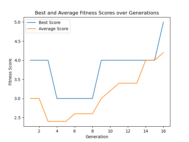
As we are done with the theoretical part it is now time to implement a real-world working example, that will find a solution to our binary digit sum maximization problem. Below you can find a code listing with full Python implementation, the implementation has max iterations set to 100, so in case of no solution the algorithm will stop. There is an earlier stopping mechanism implemented so that in case of a sum equal to five (solution found) the algorithm will stop. On each generation, we print out each chromosome’s values to the console, and if an optimal solution is found it is announced in a console together with the number of generations needed. Additionally, plotting of average and best individuals across all generations is implemented.
import random
import matplotlib.pyplot as plt

random.seed(10)   # Set random seed for reproducibility

# Genetic Algorithm parameters
POPULATION_SIZE = 5
GENE_LENGTH = 5  # Length of binary strings
MUTATION_RATE = 0.1  # Probability of mutation
GENERATIONS = 100  # Number of generations to evolve

# Generate random population of binary strings
def initialize_population(size, gene_length):
    return [[random.randint(0, 1) for _ in range(gene_length)] for _ in range(size)]

# Fitness function: Sum of the binary digits
def fitness(individual):
    return sum(individual)

# Roulette wheel selection: Select individuals based on their fitness
def selection(population, fitness_values):
    # Normalize fitness scores to 0-1 probability range to establish selection weights
    selection_weights = [chromosome_score / sum(fitness_values) for chromosome_score in fitness_values]

    # Random selection from population given the weights
    parents = random.choices(population, weights=selection_weights, k=2)

    return parents

# Single-point crossover
def crossover(parent1, parent2):
    point = random.randint(1, GENE_LENGTH - 1)  # Choose crossover point
    offspring1 = parent1[:point] + parent2[point:]
    offspring2 = parent2[:point] + parent1[point:]
    return offspring1, offspring2

# Mutation: Flip a random bit with a given probability
def mutate(individual):
    if random.random() < MUTATION_RATE:
        point = random.randint(0, GENE_LENGTH - 1)
        individual[point] = 1 - individual[point]  # Flip the bit (0 -> 1, 1 -> 0)
    return individual

# Genetic Algorithm
def genetic_algorithm():
    population = initialize_population(POPULATION_SIZE, GENE_LENGTH)
    best_scores = []
    average_scores = []

    for generation in range(GENERATIONS):
        # Calculate fitness for each individual
        fitness_values = [fitness(individual) for individual in population]

        # Record best and average fitness
        best_scores.append(max(fitness_values))
        average_scores.append(sum(fitness_values) / POPULATION_SIZE)

        # Print current generation's population and fitness
        print(f"Generation {generation + 1}:")
        for individual, fit_value in zip(population, fitness_values):
            print(f"Individual: {individual}, Fitness: {fit_value}")

        # Select parents and generate offspring through crossover
        new_population = []
        while len(new_population) < POPULATION_SIZE:
            parent1, parent2 = selection(population, fitness_values)
            offspring1, offspring2 = crossover(parent1, parent2)
            new_population.extend([mutate(offspring1), mutate(offspring2)])

        # Replace the old population with the new one
        population = new_population[:POPULATION_SIZE]

        # Check if the optimal solution has been found
        if max(fitness_values) == GENE_LENGTH:
            print(f"Optimal solution found in generation {generation + 1}!")
            break

    # Plot the results
    plt.plot(range(1, len(best_scores) + 1), best_scores, label="Best Score")
    plt.plot(range(1, len(average_scores) + 1), average_scores, label="Average Score")
    plt.xlabel('Generation')
    plt.ylabel('Fitness Score')
    plt.title('Best and Average Fitness Scores over Generations')
    plt.legend()
    plt.show()

    # Return the final population
    return population

# Run the genetic algorithm
final_population = genetic_algorithm()
print("Final Population:", final_population)
Listing output:
Generation 1:
Individual: [0, 1, 1, 0, 0], Fitness: 2
Individual: [1, 1, 1, 0, 0], Fitness: 3
Individual: [1, 1, 0, 0, 1], Fitness: 3
Individual: [0, 1, 0, 1, 1], Fitness: 3
Individual: [1, 1, 1, 1, 0], Fitness: 4
Generation 2:
Individual: [0, 1, 0, 1, 1], Fitness: 3
Individual: [0, 1, 0, 1, 1], Fitness: 3
Individual: [0, 1, 1, 0, 1], Fitness: 3
Individual: [1, 1, 0, 0, 0], Fitness: 2
Individual: [1, 1, 1, 1, 0], Fitness: 4
Generation 3:
Individual: [1, 1, 0, 0, 0], Fitness: 2
Individual: [0, 1, 1, 0, 0], Fitness: 2
Individual: [0, 1, 1, 0, 0], Fitness: 2
Individual: [1, 1, 0, 1, 1], Fitness: 4
Individual: [1, 1, 0, 0, 0], Fitness: 2
Generation 4:
Individual: [0, 1, 0, 1, 1], Fitness: 3
Individual: [1, 1, 1, 0, 0], Fitness: 3
Individual: [0, 1, 0, 0, 0], Fitness: 1
Individual: [1, 1, 1, 0, 0], Fitness: 3
Individual: [0, 1, 1, 0, 0], Fitness: 2
Generation 5:
Individual: [0, 1, 1, 0, 0], Fitness: 2
Individual: [1, 1, 1, 0, 0], Fitness: 3
Individual: [1, 1, 1, 0, 0], Fitness: 3
Individual: [1, 1, 1, 0, 0], Fitness: 3
Individual: [0, 1, 0, 0, 0], Fitness: 1
Generation 6:
Individual: [0, 1, 1, 0, 0], Fitness: 2
Individual: [1, 1, 1, 0, 0], Fitness: 3
Individual: [1, 1, 1, 0, 0], Fitness: 3
Individual: [1, 1, 1, 0, 0], Fitness: 3
Individual: [0, 1, 1, 0, 0], Fitness: 2
Generation 7:
Individual: [1, 1, 1, 0, 0], Fitness: 3
Individual: [1, 1, 1, 0, 0], Fitness: 3
Individual: [1, 1, 1, 0, 0], Fitness: 3
Individual: [0, 1, 1, 0, 0], Fitness: 2
Individual: [0, 1, 1, 0, 0], Fitness: 2
Generation 8:
Individual: [0, 1, 1, 0, 0], Fitness: 2
Individual: [0, 1, 1, 0, 0], Fitness: 2
Individual: [1, 1, 1, 0, 0], Fitness: 3
Individual: [1, 1, 1, 0, 0], Fitness: 3
Individual: [1, 1, 1, 0, 0], Fitness: 3
Generation 9:
Individual: [1, 1, 1, 0, 0], Fitness: 3
Individual: [0, 1, 1, 0, 0], Fitness: 2
Individual: [1, 1, 1, 0, 0], Fitness: 3
Individual: [1, 1, 1, 0, 1], Fitness: 4
Individual: [1, 1, 1, 0, 0], Fitness: 3
Generation 10:
Individual: [1, 1, 1, 0, 0], Fitness: 3
Individual: [1, 1, 1, 0, 0], Fitness: 3
Individual: [1, 1, 1, 0, 0], Fitness: 3
Individual: [1, 1, 1, 0, 1], Fitness: 4
Individual: [1, 1, 1, 0, 0], Fitness: 3
Generation 11:
Individual: [1, 1, 1, 0, 1], Fitness: 4
Individual: [1, 1, 1, 0, 0], Fitness: 3
Individual: [1, 1, 1, 0, 1], Fitness: 4
Individual: [1, 1, 1, 0, 0], Fitness: 3
Individual: [1, 1, 1, 0, 0], Fitness: 3
Generation 12:
Individual: [1, 1, 1, 0, 1], Fitness: 4
Individual: [1, 1, 1, 0, 0], Fitness: 3
Individual: [1, 1, 1, 0, 1], Fitness: 4
Individual: [1, 1, 1, 0, 0], Fitness: 3
Individual: [1, 1, 1, 0, 0], Fitness: 3
Generation 13:
Individual: [1, 1, 1, 0, 1], Fitness: 4
Individual: [1, 1, 1, 0, 1], Fitness: 4
Individual: [1, 1, 1, 0, 0], Fitness: 3
Individual: [1, 1, 0, 0, 0], Fitness: 2
Individual: [1, 1, 1, 1, 0], Fitness: 4
Generation 14:
Individual: [1, 1, 1, 0, 1], Fitness: 4
Individual: [1, 1, 1, 0, 1], Fitness: 4
Individual: [1, 1, 1, 0, 1], Fitness: 4
Individual: [1, 1, 1, 1, 0], Fitness: 4
Individual: [1, 1, 1, 0, 1], Fitness: 4
Generation 15:
Individual: [1, 1, 1, 0, 1], Fitness: 4
Individual: [1, 1, 1, 0, 1], Fitness: 4
Individual: [1, 1, 1, 0, 1], Fitness: 4
Individual: [1, 1, 1, 0, 1], Fitness: 4
Individual: [1, 1, 1, 0, 1], Fitness: 4
Generation 16:
Individual: [1, 1, 1, 1, 1], Fitness: 5
Individual: [1, 1, 1, 0, 1], Fitness: 4
Individual: [1, 1, 1, 0, 1], Fitness: 4
Individual: [1, 1, 1, 0, 1], Fitness: 4
Individual: [1, 1, 1, 0, 1], Fitness: 4
Optimal solution found in generation 16!
Conclusions
In this article I presented an concept of Genetic Algorithms that are part of broad ML scene. They offer a powerful and flexible yet simple to implement approach, that can be utilized in various optimization, search and combinatorics problems.